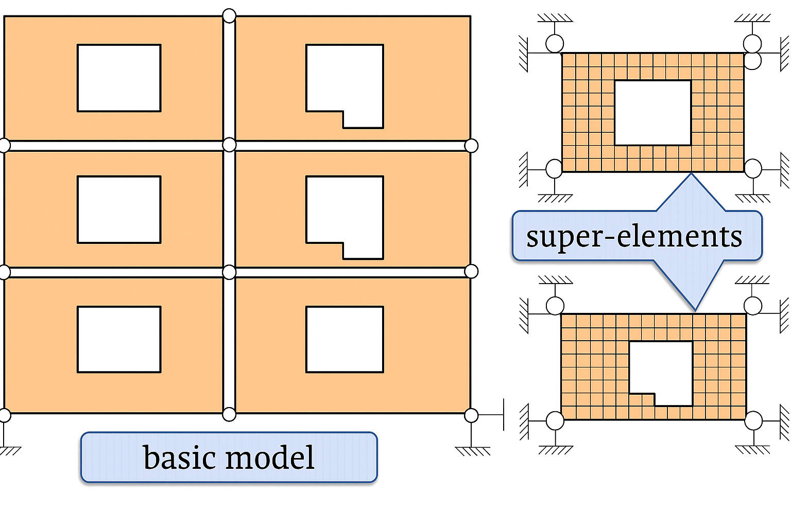
If the design model is too cumbersome, it can be convenient to organize a recursive analysis by splitting the entire system into subsystems—super-elements (SE). This approach is especially effective when the subdivision into subsystems is natural: for example, a building composed of volumetric blocks (a volumetric block is a super-element) or a high-rise diaphragm assembled from individual panels (a panel is a super-element). A fragment of a high-rise diaphragm is shown in Fig. 1a. The diaphragm consists of separate panels connected at corner nodes.
Such a system can be analyzed in the usual way: generate the required mesh and analyze the entire model at once. However, the large number of nodes, elements, and unknown displacements may significantly complicate the solution.
By using super-elements, the analysis can be carried out in stages, substantially reducing the problem size at each stage.
First, assemble the stiffness matrices for all types of super-elements (in this case, there are two types, see Fig. 1b), then analyze the system composed of these super-elements (here, the system consists of 6 super-elements with 12 super-nodes). This analysis yields the displacements of the super-nodes. At the final stage, analyze each of the six super-elements for the prescribed super-node displacements and for local loads.
a) b)
Fig. 1. Design model with super-elements: a) overall scheme; b) super-elements
The analysis sequence for a system assembled from super-elements is analogous to the standard FEM procedure, with the only difference that the stiffness matrix and the reduction of local loads to nodal loads are determined not from FEM shape functions but numerically. Since a super-element is itself a sufficiently complex system, the “shape functions” are constructed via a numerical analysis of the super-element under unit displacements of the super-nodes, resulting in an influence matrix that relates the internal node displacements of the super-element to unit super-node displacements. In this way, the super-element recursion method may be viewed as a finite element method where the shape functions are built using influence matrices.
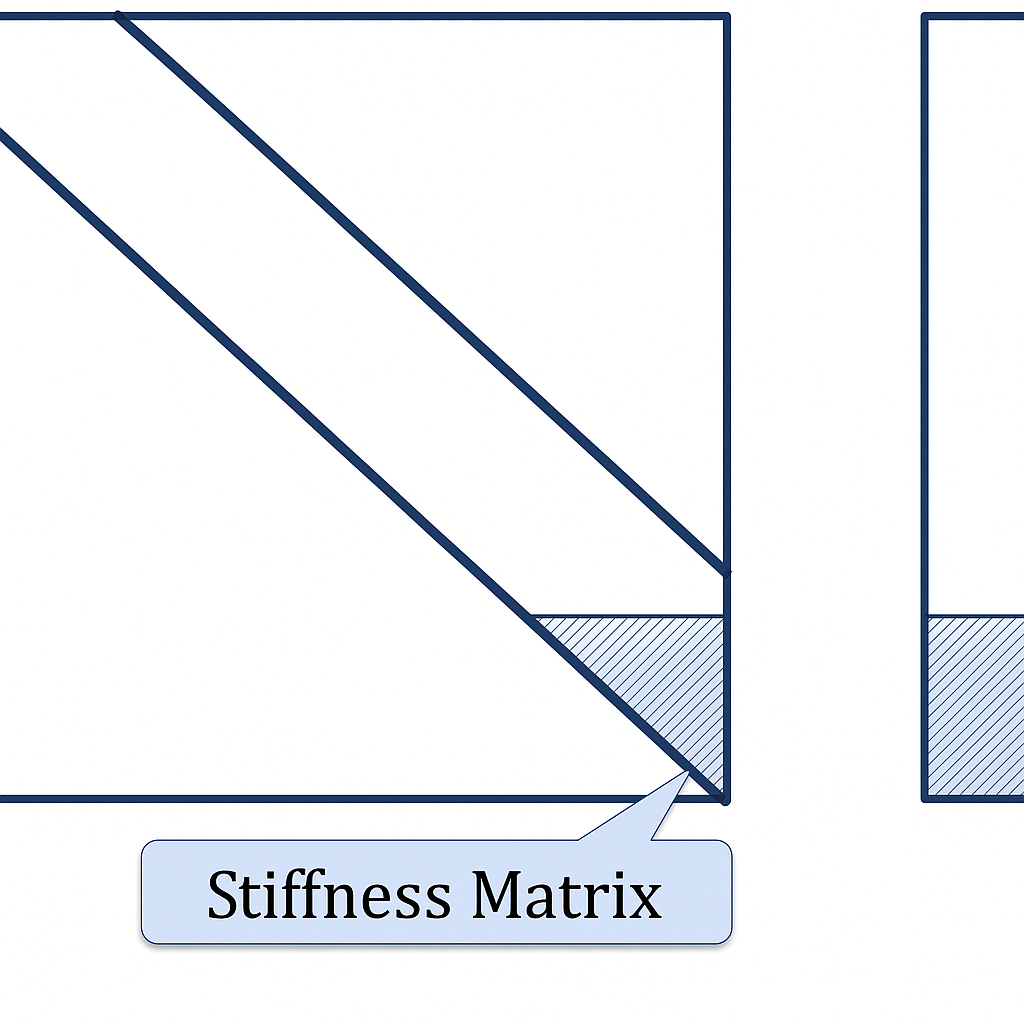
Another super-element processing procedure [3] is based on the observation that, in physical terms, eliminating the j-th unknown by Gaussian elimination corresponds to releasing the j-th constraint. This yields the following scheme for assembling the stiffness matrix and reducing local loads to nodal loads: for the i-th super-element, number all internal nodes first (let the corresponding number of degrees of freedom be ni), then the super-nodes (let the number of DOFs for the super-nodes be ni0); write the canonical equations for all ni + ni0 DOFs (Fig. 2); eliminate the ni internal unknowns; the remaining parts of the matrix and right-hand side (shaded in Fig. 2) form the desired stiffness matrix and the vector of nodal loads at the super-nodes of the super-element, to which the distributed local loads over the super-element’s domain are reduced.
The computational process can be extended by subdividing super-elements into second-rank super-elements, and so on, organizing a multi-rank recursion of the super-element method (SEM).
The main ideas of the SEM were first presented by Przheminitsky [1]. They were developed further by Meissner [2], who formalized them and generalized to multiple hierarchy levels (multi-rank recursion of SEM). Subsequent developments of SEM are presented in a series of later works [3–12].
In mathematical analogy, SEM is reminiscent of block Gaussian elimination, and its multi-rank recursion is akin to modern nested-dissection methods for sparse matrices; however, like FEM, the super-element method is based on direct discretization of the design model. In this sense, SEM is highly intuitive and natural, resembling the assembly of a structure from sections and blocks.
SEM is very effective in several cases, for example:
- for large-scale problems containing topologically identical super-elements—computations are reduced because the stiffness matrix for identical super-elements is assembled only once;
- for structural schemes where nonlinearity is localized in a limited region;
- for assembling the stiffness matrix of elements with substantial variation of stiffness properties over the element’s domain due to nonlinearity or design features (e.g., a bar with variable cross-section along its length);
- for elements interacting with a large-scale medium and connected to the main structural scheme by a single node (e.g., a pile in a soil mass).
Analysis of a structural scheme with identical super-elements
The design scheme is shown in Fig. 3.
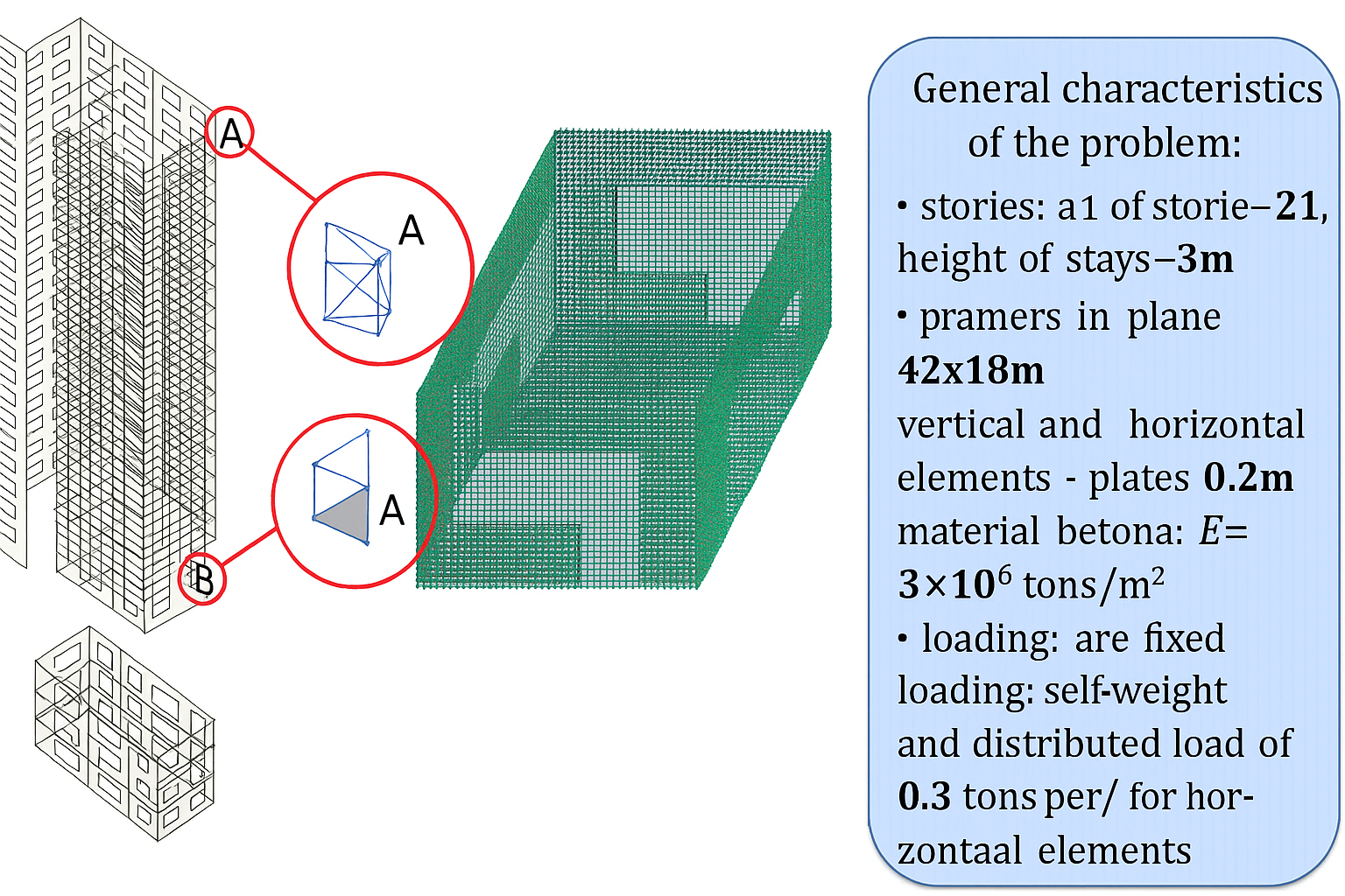
The analysis was performed in the LIRA-FEM software suite on a Pentium Core i7 (8 cores), 16 GB RAM. Two analyses were carried out (using rectangular plate finite elements): without super-elements and with super-elements.
The first design scheme contained 3,771,744 elements, 3,850,650 nodes, and 19,421,820 unknowns. The second design scheme contained 378 super-elements. Each super-element included 660 nodes.
Comparison of the two analyses is given in Table 1.
Table 1
| Compared parameters | First scheme (without SE) | Second scheme (with SE) |
| Vertical displacement at node A, mm | 177.4 | 177.4 |
| Stress in element B, kg/cm2 | −174.1 | −174.1 |
| Solution time, min* | 61 | 9 |
| *Solution time includes: assembling and solving the equations, computing internal forces in all elements, computing displacements at all nodes, and generating contour plots. | ||
The example demonstrates a significant speed-up (see Table 1). The advantages of SEM go further: it greatly simplifies input preparation and results analysis and, arguably most importantly, improves the accuracy of the solution. For very large problems with widely varying stiffness properties, the conditioning deteriorates and rounding errors accumulate, which may lead to incorrect results. In such cases, SEM is an effective tool for combating the “curse of dimensionality” inherent to most numerical methods, including FEM.
Analysis of structures with a localized nonlinear region
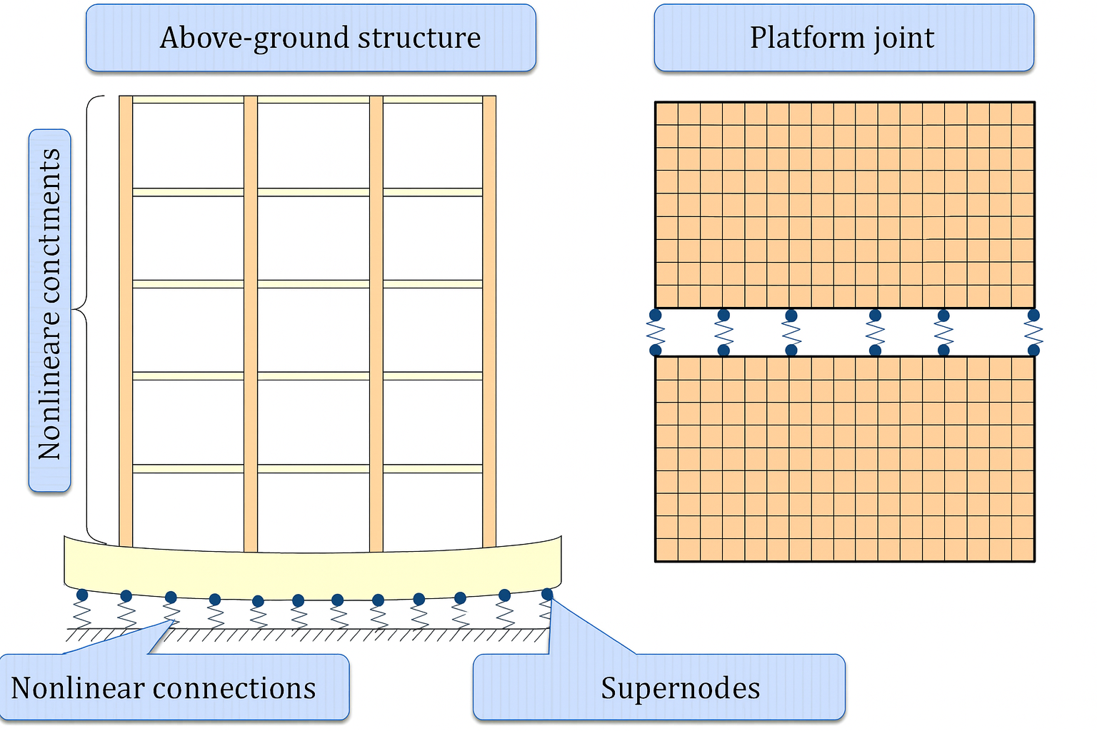
Figure 4 schematically shows a structure: a superstructure supported by connections exhibiting pronounced nonlinearity. The superstructure itself, within the required accuracy, can be analyzed in a linear setting. The superstructure model may contain many nodes and elements, and including it directly in a nonlinear analysis driven by the connections’ nonlinearity would greatly increase solution time. In this case, it is reasonable to declare the superstructure model a super-element and solve the nonlinear problem only for the main scheme comprising the super-nodes (bold dots in Fig. 4a) and the nonlinear connections.
The same approach can be used when modeling a panel building with platform joints between panels (Fig. 4b). Precast panels under service loads behave essentially linearly elastic, and the overall nonlinearity is localized in the platform joints. Introducing the panels as super-elements can therefore dramatically reduce the solution time for the nonlinear problem.
Using FEM to assemble the stiffness matrix of a bar with variable cross-section
Stiffness variation along a bar may be caused by web height changes, flange width variation, or other design features. In such cases, deriving closed-form stiffness matrices by expressing the variation of stiffness characteristics along the bar (for EIz, EIy, EA, GJ, etc.) can be difficult.
Introducing many intermediate nodes into the model is possible, but it increases the problem size and complicates input and post-processing. Here, SEM is convenient (Fig. 5).
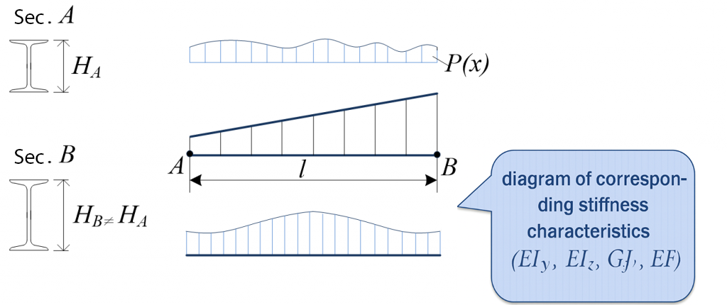
The bar is divided along its length into n segments. Nodes A and B are declared super-nodes. Following the scheme of Fig. 2, assemble the bar stiffness matrix and reduce local loads to nodal loads.
As a result, the solution of the whole system is defined by the displacements of nodes A and B. If internal node displacements are needed, a back-substitution is performed for the right-hand sides—see Fig. 2, where ni0 are the found super-node displacements at A and B—after which internal forces along the bar are obtained.
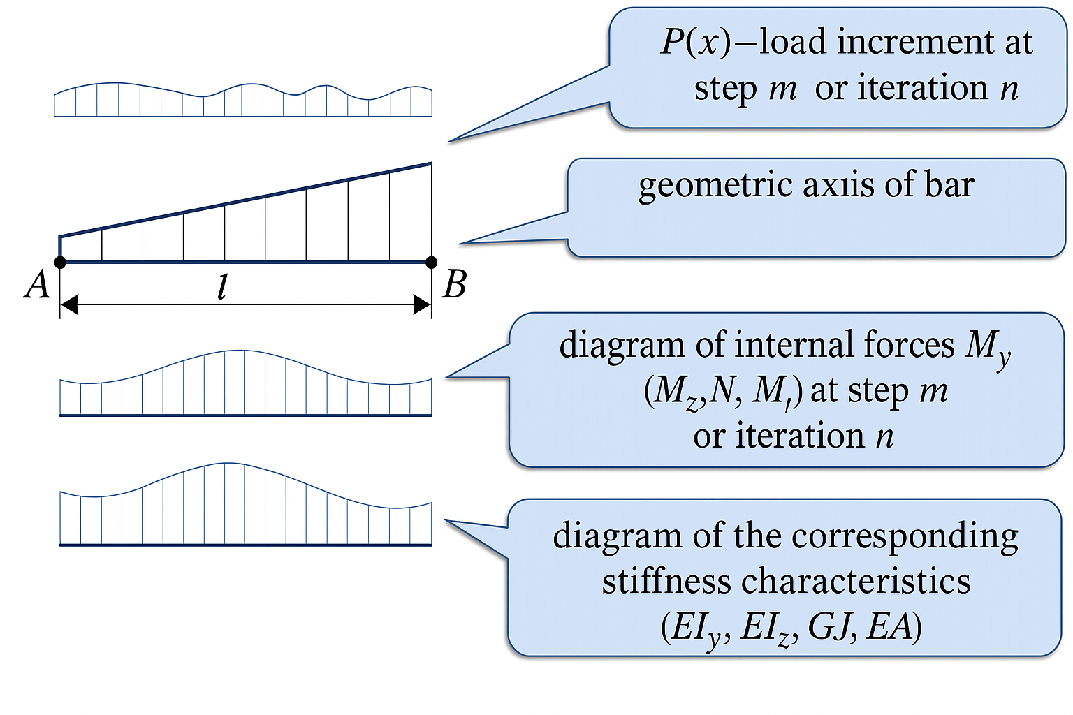
Using SEM to assemble a bar stiffness matrix for nonlinear problems
In materially nonlinear analyses, an important procedure is assembling the bar stiffness matrix at step m or iteration n. Changes of internal forces along the bar cause changes in the section stiffness properties (Fig. 6).
The task is further complicated because the centroid of the stiffness characteristics shifts relative to the geometric axis of the bar, about which the equilibrium equations are written (Fig. 7).
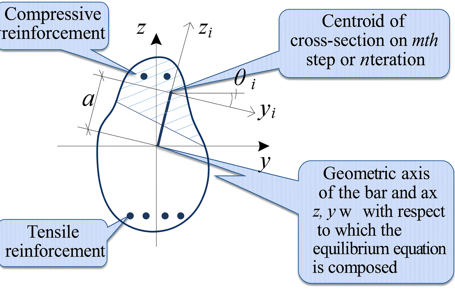
Hence, each i-th section has not only its stiffness characteristics at step m or iteration n (EIy,i, EIz,i, GJi, EAi, …), but also an Offset ai (absolutely rigid insert) and a pure rotation angle θi.
Accounting for these effects by inserting many intermediate nodes sharply increases the problem size. In this case, SEM is advisable, analogous to the procedure above for a bar with variable cross-section.
Using SEM to assemble a pile stiffness matrix within a soil mass
Pile–soil interaction(Fig. 8) can be modeled by introducing additional nodes along the pile and assigning, at these nodes, connections of finite stiffness in three directions. This approach, however, dramatically increases the problem size because the superstructure, foundation, soil mass, and piles with many intermediate nodes all have to be included in the model.
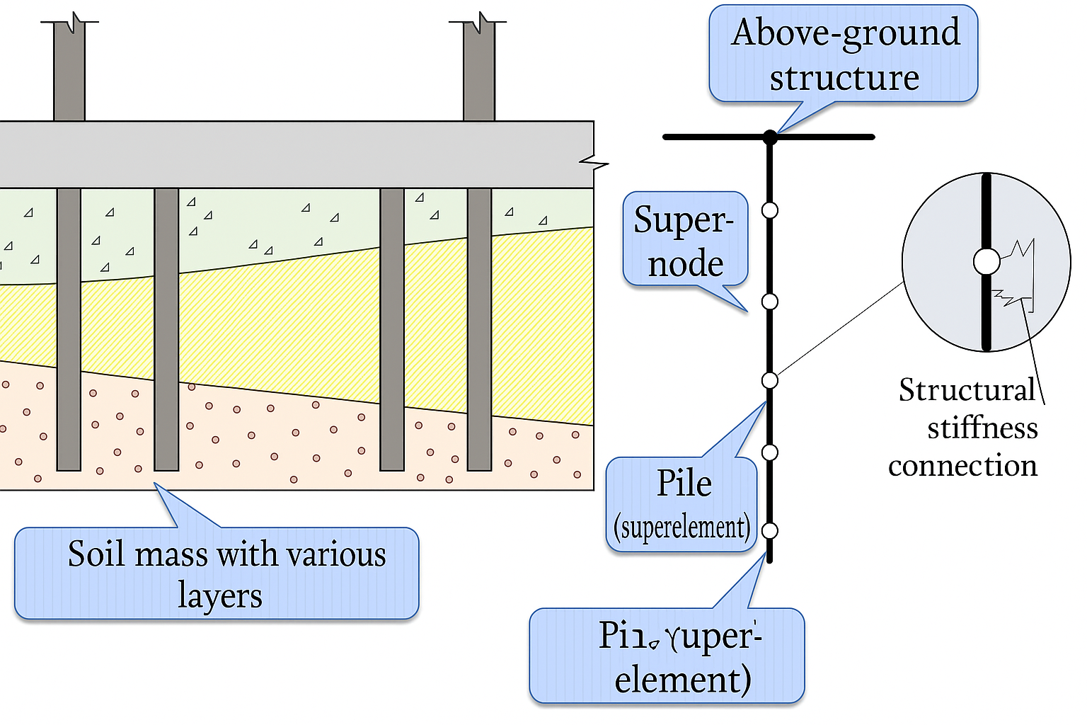
In this case, SEM is advisable. The bar (pile) has a single super-node at the pile–superstructure junction. The stiffness matrix is assembled similarly to the super-element procedure for a bar with variable stiffness, with the only difference that, at intermediate nodes, besides the bar’s own stiffness characteristics, the stiffness of the adjoining finite-stiffness connections (representing interaction with the soil layer) is also taken into account.
Thus, when solving the interaction problem of the superstructure with the soil mass, only the connections at super-nodes are modeled, and there is no need to include the full soil mass explicitly in the global model.
The implementation of SEM is fairly involved. In the former USSR, SEM was implemented in the KASKAD software suite [10], the MIRAGE software suite [11], and in all subsequent products of the LIRA family, including modern versions of LIRA-SAPR.
References
- Przheminitsky, E. S. Matrix method for structural analysis based on substructuring. Rocket Technology and Astronautics, 1963, No. 1.
- Meissner, K. Multi-connected assembly algorithm for the stiffness method of structural analysis. Rocket Technology and Astronautics, 1968, No. 11.
- Gorodetsky, A. S. Numerical implementation of the finite element method. In: Strength of Materials and Structural Theory. Kyiv: Budivelnyk, 1973, Vol. XX.
- Gorodetsky, A. S. Computing suite for analyzing building structures on the MINSK-32 computer. In: Organization, Methods, and Technology of Design, 1976, Issue 9.
- Nagy, L. I. Static Analysis via Substructuring of an Experimental Vehicle Front-End Body Structure. Intern. Conf. on Vehicle Structural Mechanics: Finite Element Application to Vehicle Design, Detroit, Michigan, 1974 (March).
- Neke, I., Nagai, K., Fuke, H. General-purpose program of plane stress analysis by FEM and its application. IHI Engineering Review, 1972, Vol. 5, No. 1.
- Araldesen, P. O., Roren, E. M. Q. The Finite Element Method Using Super-elements. SESAM-69 Struct., Conf. on Modern Techniques of Ship Structural Analysis and Design. Berkeley: University of California, 1970 (September).
- Super-element method in strength analysis of ship structures / V. A. Postnov, S. A. Dmitriev, B. K. Eltyshev, A. A. Rodionov. Sudostroenie, 1975, No. 11.
- Postnov, V. A., Rodionov, A. A., Tsenkov, M. Ts. Super-element method in linear and nonlinear problems. In: Finite Element Method in Structural Mechanics. Gorky: GGU Press, 1975.
- Postnov, V. A., Dmitriev, S. A., Eltyshev, B. K., Rodionov, A. A. Super-element method in the analysis of engineering structures. Leningrad: Sudostroenie, 1979.
- Gorodetsky, A. S. MIRAGE program for static structural analysis by FEM. In: Proc. All-Union Conference “Design Automation as a Comprehensive Problem of Improving National Design Practice”. Moscow, 1973.
- Gorodetsky, A. S. On the applicability of super-elements to various problems of structural mechanics. Structural Mechanics and Analysis of Constructions, 2015, No. 4, pp. 51–56.
If you find a mistake and want to inform us about it, select the mistake, then hold down the CTRL key and click ENTER.

Comments